The finite element method is a powerful numerical technique that is used to obtain approximate solutions to problems that are governed by differential equations. It has many applications in engineering, but is most commonly used to perform structural analysis, to solve heat transfer problems, or to model fluid flow.
This page will describe how the finite element method (FEM) is used to perform stress analysis, but the same principles can be applied to other analysis types. A lot of the information on this page is summarised in this video:
Nodes and Elements
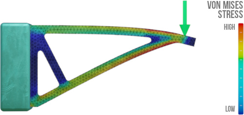
The finite element method approaches the difficult task of solving the equations governing a continuous system (e.g. the static equilibrium equations for a static stress analysis problem or the heat transfer equations for a heat transfer problem) by splitting the body being analysed into a collection of small elements, that are connected together at nodes. This process is called discretisation and the collection of elements and nodes is called the finite element mesh.
The finite element method will determine an approximate solution to the stress analysis problem using the discretised mesh, which is much easier than determining an exact solution for the continuous system.
Element Types
Finite element analysis (FEA) software packages provide hundreds of different element types for the user to choose from. Most fit into one of the following three categories:
- Line elements are used to model one-dimensional structures like beams, rods or pipes. The geometry of the element cross-section is defined by the user.
- Surface elements are used to model thin surfaces like shells. The thickness of the element is defined by the user.
- Solid elements are used to model three-dimensional bodies.
The most common surface elements are triangular (TRI) or quadrilateral (QUAD) elements. The most common solid elements are tetrahedral (TET) and hexahedral (HEX) elements, although wedge- and pyramid-shaped elements can also be used.

Complex geometries can often only be meshed using tri and tet elements. Quad and hex elements are best suited to regular geometry, where they are preferred to tri and tet elements because they are more efficient and require fewer nodes.
Elements don’t vary only based on their shape – two elements can have the exact same shape but have completely different formulations that make them suitable for different analysis types, because they correspond to different assumptions and different modelling approaches. Here are a few examples:
- Plane stress elements are 2D surface elements that are designed to be used for plane stress conditions.
- Plane strain elements are 2D surface elements that are designed to be used for plane strain conditions.
- Pipe elements are 1D line elements that are used to model pipes – they differ from beam elements because they capture the effect of internal and/or external pressure in the element formulation.
The best element type will depend on the problem being analysed. Often it is best to use a modelling approach that simplifies the problem as much as possible while providing reasonable results. Say that you need to analyse a pipeline being subjected to loads caused by a landslide. You might choose to model the pipeline using pipe elements if you are only interested in the general displacement of the pipeline. But if you need to model how the pipeline cross-section deforms locally, you might need to use shell or even solid elements that model the three-dimensional geometry of the pipeline.
Linear vs Quadratic Elements
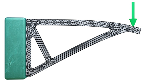
Elements can be linear (also known as first-order elements) or quadratic (second-order elements). Quadratic elements have additional mid-side nodes along each side of the element. They require more computational power but generally produce more accurate results than linear elements.
Linear tetrahedral elements (e.g. TET4, a 4-noded tetrahedral element) are known to exhibit overly stiff behavior, and their use should be avoided – TET10 quadratic tetrahedral elements should usually be used instead.
The Efficient Engineer Summary Sheets
The Efficient Engineer summary sheets are designed to present all of the key information you need to know about a particular topic on a single page. It doesn’t get more efficient than that!
Degrees of Freedom
Each node in the finite element mesh has a certain number of degrees of freedom. In a two-dimensional stress analysis for example each node will have 3 degrees of freedom – translation in the X and Y axes, and rotation about the Z axis. For thermal analysis each node will have a single degree of freedom, which is the nodal temperature.
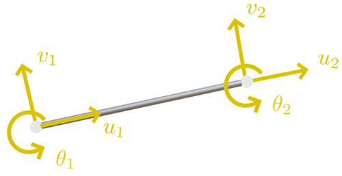
For each element in the mesh a vector $ \left \{ u \right \}$ is defined that stores all of the degrees of freedom for that element. A beam element in a two dimensional analysis for example will have six degrees of freedom in total (three at each node), so $ \left \{ u \right \}$ will look like this:
$$ \left \{ u \right \} = \begin{Bmatrix}u_1\\v_1\\ \theta_1\\u_2\\v_2\\ \theta_2 \end{Bmatrix}$$
The Element Stiffness Matrix
Each element in a mesh has a certain amount of stiffness, that essentially defines how much the nodes of the element will displace when acted upon by forces. This behaviour can be represented by the equation shown below:
$$\left \{ f \right \} = [k] \left \{ u \right \}$$
The displacements (translations and rotations) in the nodal displacements vector $ \left \{ u \right \}$ depend on the nodal forces vector $ \left \{ f \right \}$ that contains the loads (forces and moments) acting on the element nodes, and on the element stiffness matrix $[k]$.
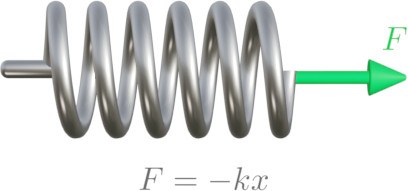
This is analogous to Hooke’s law for a spring, where the spring displacement $x$ depends on the applied force $F$ and the spring stiffness $k$.
The element stiffness matrix depends on the type of element being used. The element stiffness matrix for the 2D beam element mentioned earlier is shown below. The terms in the matrix depend on the beam geometry and material – $A$ is the area of the beam cross-section, $E$ is the Young’s modulus of the beam material, $I$ is the second moment of area of the beam cross-section and $L$ is the length of the beam element.

The element stiffness matrix is always a square matrix – the number of rows and the number of columns are equal to the number of degrees of freedom of the element.
How the Element Stiffness Matrix Is Derived
The element stiffness matrices for different element types are defined in the FEA software being used – they don’t need to be derived by the user. But it is still a good idea to understand where they come from.
The element stiffness matrix for a specific element is derived from the equilibrium equations that govern the behaviour of that element. These governing equations are usually differential equations. For example the deflection of a beam is governed by the equation shown below. You can visit our page on beam deflections if you’d like to learn where this equation comes from.
$$EI \frac{d^4 v(x)}{dx^4} = q(x)$$
This is quite a simple governing equation, but for more complex elements the equations are much less straightforward. In these cases the governing equations are usually expressed in what is called the weak form, where the differential equation is expressed as an integral. Solving the weak form of the governing equation yields an approximate solution to the equation, but is easier than trying to solve the governing differential equation itself.
Two common methods for deriving and solving the weak form of the governing equations are:
- the Principle of Minimum Potential Energy
- the Galerkin Method of Weighted Residuals
Shape Functions
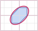
For these methods to be applied, there needs to be a way of defining how displacements and other field variables (like stress or strain) are defined within the element, instead of just at the nodes of the element.
To do this, interpolation functions called shape functions are defined that interpolate the values of a variable at the nodes of an element to provide values anywhere within the element. The shape functions are just assumed functions – polynominals are often used because they are relatively simple to compute and are sufficiently accurate.
The Global Stiffness Matrix
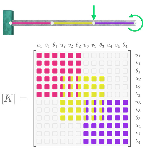
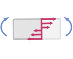
Once the element stiffness matrices for all of the elements in a mesh have been defined, they can then be assembled to create a huge global stiffness matrix $[K]$ that represents the stiffness of the entire structure. One node can obviously be connected to multiple elements, so the stiffness terms that apply for a specific degree of freedom can have contributions from multiple different element stiffness matrices. This means that the way the element stiffness matrices are assembled depends on how the elements of the mesh are connected to each other.
The image below illustrates how the global stiffness matrix is assembled for a simple cantilever beam model that has three elements and four nodes. In practice FE models often have hundreds of thousands of nodes and elements, so the resulting matrix is very large.
The Global FEM Equation
The global FEM equation describes the relationship between the forces and moments acting on all of the nodes in the mesh $ \left \{ F \right \}$, the displacements and rotations at all of the nodes in the mesh (i.e. all of the degrees of freefom) $ \left \{ U \right \}$, and the global stiffness matrix $[K]$.
$$[F] = [K] \left \{ U \right \}$$
The nodal displacements and rotations $\left \{ U \right \}$ are the unknowns that we are trying to determine.
Before solving this equation the vector of nodal forces $\left \{ F \right \}$ needs to be filled in with any of the known external loads, and the vector of nodal displacements $\left \{ U \right \}$ needs to be filled in with any boundary conditions. Boundary conditions are known displacements at specific nodes – if a node is fully fixed for example, the degrees of freedom in $\left \{ U \right \}$ corresponding to displacements and rotations at that node will be equal to zero.
Solving the Global FEM Equation
One typical approach that could be used to solve an equation of the form $[F] = [K] \left \{ U \right \}$ would be to invert the global stiffness matrix $[K]$ and solve for $\left \{ U \right \}$. However this would likely be quite difficult for a sizeable model, and it would also be inefficient because the global stiffness matrix is very large and is also sparse (meaning that it contains a lot of zeros).
Instead commercial solvers mostly use methods that involve iteratively approximating the displacement vector, like the conjugate gradient method, to solve the global FEM equation.
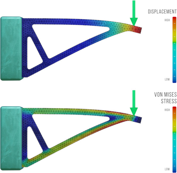
Stresses and Other Outputs
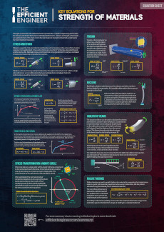
Solving the global FEM equation provides the displacements (translations and rotations) at each node in the mesh. These displacements can be used to calculate the strains in each of the elements, and from there other outputs like principal stresses or von Mises stresses can be determined.
Summary of How the Finite Element Method Works
The process of applying the finite element method to perform stress analysis can be summarised by the 7 steps listed below. When working with Finite Element Analysis (FEA) software, some of these steps are performed by the user (e.g. defining the loads and boundary conditions), and some are performed by the software (e.g. defining the element stiffness matrices, and solving the global FEM equation).
STEP 1 | Problem definition
The problem is defined, which includes defining the body being analysed, its material properties, and the loads and boundary conditions acting on it.
STEP 2 | Discretisation
The body is discretised as a collection of nodes and elements to create a mesh.
STEP 3 | Element Stiffness Matrix Definition
For each element in the mesh an element stiffness matrix $[k]$ is defined that describes how the nodes of the element will displace for a set of applied loads.
STEP 4 | Global Stiffness Matrix Definition
The element stiffness matrices for all of the elements in the mesh are assembled together to form a global stiffness matrix $[K]$ based on how the elements are connected together.
STEP 5 | Global FEM Equation Definition
The global FEM equation $\left \{ F \right \} = [K] \left \{ U \right \}$ that describes how all of the nodes in the model will displace for a set of applied loads is defined based on the global stiffness matrix $[K]$.
STEP 6 | Solving the Global FEM Equation
The global FEM equation is solved using computational methods based on the applied loads and boundary conditions that have been defined. This provides the translations and rotations $\left \{ U \right \}$ at each node of the mesh.
STEP 7 | Determining the Required Outputs
Strains, stresses and other desired outputs can be determined based on the calculated nodal displacements.
Well done for making it this far! You should now hopefully have a good understanding of how the finite element method works.
Related Topics
Stresses in Beams
Shear and normal stresses are generated in a beam due to externally applied loads and the way the beam is supported.
Failure Theories
Failure theories like the von Mises and Tresca theories are used to predict the conditions that will results in the failure of a material.